Audit First Redshift Cost Optimization for Cloud Architects

Right now, three levers move a Redshift bill more than anything else: right-sizing compute (RA3 or RG, plus reservations), cutting unnecessary Spectrum scans, and enforcing workload controls through WLM and query monitoring rules. Fix those three, and you’ve typically addressed the bulk of a bloated bill. Everything else, snapshots, encoding, distribution keys, is real money too, but it moves the needle less per hour invested.

---

TL;DR:

• Most cost savings come from right-sizing compute, reducing Spectrum scans, and controlling workload queues, which can cut the bulk of your bill.
• Pick the appropriate pricing model based on workload stability: provisioned, serverless, or Spectrum, and test configurations during peak usage before committing.
• Optimizing Spectrum costs involves data partitioning, switching to columnar formats, and avoiding unnecessary data scans; query analysis can reduce scan volume by 70-90%.
• Using WLM and query monitoring rules helps prevent runaway queries, while setting conservative snapshot retention and archiving cold data reduces unnecessary storage costs.
• Conducting regular audits with tools like Redshift Advisor and Cost Explorer can reveal the top cost drivers, often enabling up to 70% reduction in Spectrum and query-related expenses.

---

Table of Contents

• What drives redshift cost optimization: pricing models explained
• How do you right-size Redshift compute without guessing?
• Does Redshift Serverless actually save money?
• How much does Redshift Spectrum actually cost you?
• How do WLM and QMR keep query costs from spiraling?
• What’s the right snapshot and retention policy for cost control?
• What should you monitor to keep Redshift spend under control?
• Your prioritized Redshift cost reduction checklist
• What do encoding choices really cost you in Redshift?
• Is compressing Redshift storage worth the performance hit?
• How do distribution styles and sort keys change your bill?
• Which query patterns actually reduce compute usage?
• How do data loading choices affect Redshift costs?
• Why an audit-first approach finds savings teams miss
• How Cost Beacon accelerates Redshift savings
• Sources

What drives redshift cost optimization: pricing models explained

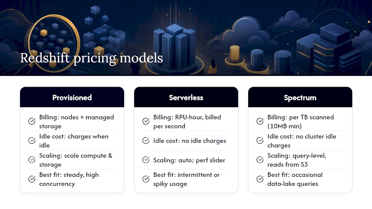
Redshift bills you in three distinct ways, and picking the wrong model for a given workload is where most teams overpay. Provisioned clusters charge for compute nodes plus managed storage. RA3 nodes separate compute from storage (you pay for compute and for storage independently, scaling each on its own), while the older DC2/DS2 style RG-adjacent instances bundle both. AWS now steers most new workloads toward RA3, though instance-store options remain relevant for smaller, storage-light jobs.

Redshift Serverless bills by RPU-hour (Redshift Processing Units), with usage measured per second and no idle charges when the warehouse is paused. A price-performance slider lets you bias the engine toward lower cost or faster runtimes, and reserved capacity is available for teams that want serverless flexibility with provisioned-style budget predictability.

Redshift Spectrum charges per terabyte scanned from S3, rounded up with a 10MB minimum per query, tracked through SVL_S3QUERY_SUMMARY.

Pick provisioned for steady, predictable, high-concurrency workloads. Pick serverless for intermittent or spiky usage where idle compute would otherwise sit unused. Pick Spectrum, carefully, for occasional queries against data-lake data you don’t want to load into the cluster at all.

How do you right-size Redshift compute without guessing?

Right-sizing starts with a hard truth: most clusters are provisioned for a peak load that happens twice a month, and the rest of the time you’re paying for idle headroom. RA3 nodes are the default recommendation for new clusters needing to scale storage independently of compute, but Graviton-based RG instances often deliver better price-performance for CPU-bound, standard-sized workloads, which is why AWS Well-Architected guidance calls out Graviton as a first check before defaulting to RA3.

To decide between on-demand and reserved pricing, look at actual usage history rather than guessing at future need. A 30 to 90 day usage analysis lets you model reserved savings against flexibility realistically. If usage is stable, a one-year reserved instance often pays for itself within months. If it’s noisy, a convertible reservation or a split approach, baseline capacity reserved plus burstable on-demand, limits your downside.

Before committing, test:

• Spin up a like-for-like test cluster and run your real, representative queries against it, not synthetic benchmarks.
• Compare cost-per-query and total runtime across RA3 and RG configurations side by side.
• Track how VACUUM and ANALYZE operations affect both runtime and disk consumption under load.
• Confirm the cluster holds 30 to 40% free disk space after your heaviest maintenance window, not just at idle.

Pro Tip: Run your test workload during your actual peak hour, not a quiet Tuesday morning. A cluster that looks right-sized at 10 AM can fall over during the Monday morning BI rush, and that’s exactly the scenario a smaller reserved commitment won’t forgive.

Does Redshift Serverless actually save money?

It depends entirely on your usage pattern, and the honest answer for most teams running steady, predictable ETL is no, it doesn’t. Serverless earns its keep on intermittent workloads, dev/test environments, or unpredictable analytical bursts where a provisioned cluster would sit half-idle most days.

The price-performance slider is the control most teams underuse. Sliding toward “optimize for cost” deliberately trades some query speed for a flatter, more predictable bill, a legitimate posture when budget stability matters more than shaving seconds off a dashboard refresh. Sliding toward performance does the opposite, and it can quietly double your RPU consumption during traffic spikes if nobody’s watching.

To keep serverless costs from surprising you:

• Set explicit RPU limits (base and max) rather than leaving scaling unbounded.
• Use reserved capacity for serverless once usage stabilizes, to lock in a predictable rate.
• Log RPU-hour consumption daily and compare it against a rolling seven-day average.
• Set a CloudWatch alarm on RPU usage spikes before they show up on next month’s invoice, not after.

How much does Redshift Spectrum actually cost you?

Spectrum bills per terabyte of data scanned from S3, and the mechanics matter more than people assume: each query rounds up to the nearest megabyte scanned, with a 10MB minimum charge even for a query that touches almost nothing. Run that math against thousands of daily queries and the rounding alone adds up.

The real number to watch: teams that apply partition pruning and query optimization to their highest-cost Spectrum queries have cut scan volumes by 70 to 90%, often with payback inside the first billing cycle.

Here’s the practical sequence for getting there:

1. Partition your data by the dimensions your queries actually filter on, usually date, region, or category, and aim for a partition hit ratio above 80%. Partitions sized between 100MB and 1GB balance scan efficiency against S3 request overhead.
2. Switch to columnar formats. Parquet or ORC files support predicate pushdown and column pruning, meaning Redshift Spectrum reads only the columns and row groups a query actually needs, not the whole object.
3. Kill SELECT * in production. Every unnecessary column pulled from S3 is billed the same as a column you actually needed.
4. Measure what’s actually being scanned. Query SVL_S3QUERY_SUMMARY directly to compute scanned bytes per query, convert to terabytes, and multiply against your per-TB rate to see exactly where the money’s going.
5. Alert on outliers. A single unfiltered join against an unpartitioned table can scan more data in one run than a well-tuned pipeline does all week. Flag any query scanning above a defined threshold and route it for review before it runs again.

Governance matters here as much as the technical fix. Treat Spectrum as a pay-per-scan engine, because that’s literally what it is, and a handful of ungoverned analysts can generate scan costs disproportionate to the entire rest of your warehouse spend.

How do WLM and QMR keep query costs from spiraling?

Workload Management (WLM) queues let you separate heavy ETL jobs from time-sensitive BI dashboards, so a single runaway transformation job doesn’t starve every analyst’s Tableau refresh of compute. Give ETL its own queue with generous memory and a lower priority, and give BI queries a smaller, faster queue that stays responsive even when batch jobs are running.

Query Monitoring Rules (QMR) enforce that isolation automatically. You can configure a rule to abort any query exceeding a runtime or row-scan threshold, or simply log it for review without killing it, useful when you’re still profiling what “normal” looks like before you start cutting queries off.

Concurrency scaling adds its own cost dimension. Each RA3 cluster earns one free hour of concurrency scaling credit per day, and usage beyond that free credit is billed per second. That’s usually fine for occasional bursts, but a cluster that’s chronically under-provisioned will burn through its daily credit fast and start racking up per-second charges every single day.

• Set usage quotas on concurrency scaling so it doesn’t become a silent, unbounded expense.
• Require query templates or review for any ad hoc query touching your largest tables.
• Build cost-aware SQL habits into onboarding: explicit column lists, partition filters, and LIMIT clauses during exploration.

Pro Tip: Log every QMR abort event for thirty days before tightening thresholds further. You’ll often find the same three dashboards or the same analyst’s scratch queries account for most violations, which tells you exactly where to focus training instead of tightening rules for everyone.

What’s the right snapshot and retention policy for cost control?

Snapshots are convenient and quietly expensive if left unmanaged. Automated snapshots accumulate storage charges the moment retention windows run longer than actual recovery needs require, and manual snapshots taken “just in case” before a migration have a habit of never getting deleted.

Keep the minimum number of manual snapshots your recovery policy actually demands, and set automated snapshot retention to match your real recovery point objective, not a default that’s been sitting untouched since cluster creation.

For colder data, don’t keep it sitting in expensive managed storage:

• Archive infrequently queried data to S3 and access it through Spectrum when someone actually needs it.
• Consider a dedicated history schema for aged records instead of leaving them in your primary tables at full compute-tier cost.
• Enable automatic table optimization so Redshift adjusts sort and distribution behavior without manual tuning cycles.
• Schedule VACUUM and ANALYZE during defined maintenance windows rather than letting them run reactively during business hours.
• Trim CloudWatch and S3 log retention to what compliance actually requires, and compress logs you do keep.

What should you monitor to keep Redshift spend under control?

Amazon Redshift Advisor is the first stop for any cost review. It analyzes live cluster usage and ranks recommendations, distribution key changes, sort key adjustments, compression opportunities, by expected impact, and it now extends across data-sharing and multi-cluster setups, surfacing fixes that benefit an entire data mesh rather than one isolated cluster.

Work Advisor’s list top to bottom by projected savings, not by whichever fix looks easiest.

For billing visibility, Cost Explorer and AWS Budgets need to be filtered correctly, since filtering by S3 will misattribute Spectrum charges entirely. Filter by the Redshift service and group by the DataScannedInTB API operation to isolate Spectrum spend cleanly from compute costs.

• Query SVL_S3QUERY_SUMMARY weekly to track scanned bytes trends, not just totals.
• Pull STL system tables to identify your heaviest queries by runtime and row count.
• Track partition hit ratio as a standing metric, not a one-time audit item.
• Set AWS Budgets alerts at 70% and 90% of your monthly Redshift allocation.

Fixing the top five most expensive queries or tables in a cluster typically resolves 60 to 70% of Spectrum and query-related costs, which is why that’s always the first place to look, not the last.

Your prioritized Redshift cost reduction checklist

Cost work fails when it’s treated as one giant project instead of a sequence of small, provable wins. Here’s the order that actually works:

1. Within 48 hours: Turn on Redshift Advisor and read every recommendation. Identify your five most expensive queries by scan volume or runtime. Set a Spectrum usage quota and tighten default WLM queue settings so nothing runs unbounded while you investigate further.
2. Within one to four weeks: Roll out partition keys on your highest-scan tables. Move cold, rarely queried data to S3 and validate access through Spectrum. Test RA3 to RG migration on a staging cluster. If usage has been stable for 30 to 90 days, apply reserved purchases.
3. Within one to three months: Run full workload tests on a dedicated test cluster before finalizing any instance-family change. Implement query governance, templates, review gates, cost-aware SQL standards. Automate monitoring and alerting so this doesn’t become a quarterly fire drill again.

KPI	What it tells you
Monthly Spectrum terabytes scanned	Whether partition and format fixes are actually reducing scan volume
Percentage of queries using partition filters	Whether partition pruning discipline is holding across teams
Average bytes scanned per query	Whether query patterns are improving or quietly regressing
Percentage cost reduction month over month	Whether the whole program is translating into real invoice impact

What do encoding choices really cost you in Redshift?

Column encoding decides how much physical disk Redshift needs to store your data, and disk footprint is directly tied to managed storage billing on RA3 clusters. Poorly encoded columns don’t just cost more to store, they cost more to scan, since I/O scales with the bytes actually read off disk.

Redshift’s automatic compression analyzer picks a reasonable encoding at load time for most columns, and for the majority of workloads that default is good enough to leave alone. Where it matters is on your largest fact tables. A low-cardinality column encoded with a generic scheme instead of a targeted one like AZ64 or byte-dictionary encoding can inflate storage by a meaningful margin across billions of rows, and that inflation compounds every time the column gets scanned in a query.

The trade-off worth understanding: more aggressive encoding reduces disk footprint and I/O, but re-encoding an existing large table means an expensive ALTER TABLE ENCODE operation, or a full table rebuild in older Redshift versions. That’s not a change to make casually on a table your BI team queries constantly during business hours.

Practical approach: let automatic compression handle new tables, then run Redshift Advisor’s encoding recommendations against your existing largest tables and act only on the ones flagged with meaningful projected savings. Encoding tuning is a background task, not a first-week priority, but it’s cumulative dead weight if ignored entirely for years.

Is compressing Redshift storage worth the performance hit?

Compression in Redshift almost always saves money on managed storage, but the real trade-off shows up in CPU cycles spent decompressing data during query execution, not in the storage savings themselves.

Higher compression ratios shrink your storage bill and reduce the physical I/O a query needs to perform, which usually makes scans faster, not slower, since less data has to move off disk. The catch appears on compute-constrained clusters running CPU-intensive aggregations, where decompression overhead on very large scans can eat into the RPU or node-hour budget you were trying to protect.

For most analytical workloads, this isn’t a close call: compression wins. Storage costs money every single hour a table exists; decompression costs a marginal amount of compute only when that table is actually queried. A cold archive table sitting mostly unused should always be compressed as aggressively as possible.

Where it gets nuanced is on your hottest, most frequently scanned tables under real concurrency pressure. If a table backs a dashboard refreshed every few minutes by dozens of analysts, test compression settings against actual query latency rather than assuming maximum compression is automatically correct. Redshift Advisor’s compression recommendations already account for this balance, factoring in observed query patterns rather than storage size alone, which is one more reason to treat Advisor’s ranked list as a starting point rather than running compression analysis manually from scratch.

How do distribution styles and sort keys change your bill?

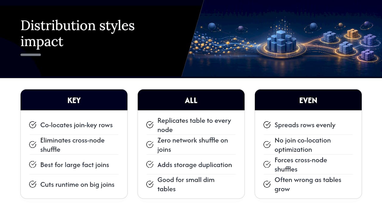
Distribution style decides which node stores which rows, and getting it wrong means queries constantly shuffle data across the network between nodes, a cost that shows up as slow runtimes and, on provisioned clusters, as compute time you’re paying for regardless of whether the query needed it.

KEY distribution, joining large fact tables on a shared distribution key, eliminates that cross-node shuffle for the joins that use it, often cutting query runtime dramatically on multi-billion-row tables. ALL distribution replicates a small dimension table to every node, which trades some storage duplication for zero network shuffle on joins against it, a fair trade for tables under a few million rows. EVEN distribution, the default fallback, spreads rows evenly with no join optimization at all, and it’s frequently the wrong choice left in place by accident on a table that’s grown large enough to matter.

Sort keys determine how much data a scan has to touch before it finds what a query is actually filtering on. A well-chosen compound sort key on your most common filter column, typically a date, lets Redshift skip entire blocks of data it knows can’t match, which reduces both I/O and, indirectly, RPU consumption on serverless. An unsorted or poorly sorted table forces a full scan every time, the query equivalent of leaving Spectrum’s partition pruning turned off.

Redshift Advisor flags both distribution and sort key mismatches directly, ranked by the runtime and cost impact of fixing each one, which makes it the fastest place to find where a schema decision made two years ago is quietly costing money today.

Which query patterns actually reduce compute usage?

Query optimization for cost, not just speed, comes down to reducing the volume of data Redshift has to touch and the number of times it has to touch it twice.

Filtering early matters more than almost anything else. A WHERE clause applied before a join lets Redshift discard irrelevant rows before they ever hit the expensive part of the execution plan, instead of joining everything and filtering afterward. Selecting only the columns a query actually needs, rather than SELECT *, reduces both memory pressure and the data volume moved between nodes during execution.

Materialized views deserve more attention than most teams give them. A dashboard query that recalculates the same aggregation from scratch every few minutes is burning compute repeatedly for a result that barely changes; a materialized view computes it once and serves cached results until a refresh is genuinely needed.

Avoid cross-joins and unfiltered joins on large tables entirely, they’re one of the fastest ways to generate a query that scans far more rows than the result set ever needed. And watch nested subqueries: a query with several layers of subqueries often performs far worse than the same logic rewritten as a single query with proper joins and window functions, because each nested layer can force an intermediate result set to materialize before the next step even starts.

How do data loading choices affect Redshift costs?

Loading data inefficiently is one of the most overlooked cost drains in a Redshift environment, because the cost shows up as compute time during ingestion, not as a line item anyone reviews separately.

COPY from S3 in parallel, using multiple evenly sized files rather than one large file, lets Redshift’s nodes load data concurrently instead of funneling everything through a single stream. A single 50GB file loads dramatically slower, and burns more compute time doing it, than the same data split across a few dozen evenly sized files.

Compressing source files before loading (Gzip or Parquet, depending on your pipeline) reduces both transfer time from S3 and the I/O Redshift needs during ingestion. Running frequent small INSERT statements instead of batched loads is another common trap, each individual insert carries transaction overhead that batched loading avoids entirely, and at scale that overhead adds up to real compute cost.

Finally, avoid loading data you don’t need yet. Staging tables that sit fully loaded for weeks before anyone queries them are paying storage costs for zero business value in the meantime. A load schedule aligned to actual consumption, not “just in case someone asks,” keeps both compute and storage spend proportional to real usage.

Why an audit-first approach finds savings teams miss

Most in-house teams can execute every fix in this playbook. What they usually lack is the time to run a full audit across every cluster, every query pattern, and every Spectrum scan simultaneously, while still shipping their actual roadmap. That’s the gap an external, audit-first review closes. Cost Beacon’s engagements have delivered an average 32% bill reduction across clients spanning fintech to telecom, precisely because a dedicated audit surfaces the full prioritized list at once, rather than one fix at a time over six months. Expect a ranked action plan with projected savings per item, and optional support implementing it.

— Aaditya Parashar

How Cost Beacon accelerates Redshift savings

An external service offering pay-on-savings AWS audits can help find the biggest money leaks first, so you fix the highest-impact ones without spending your own engineering weeks chasing every Spectrum scan and idle RA3 node yourself.

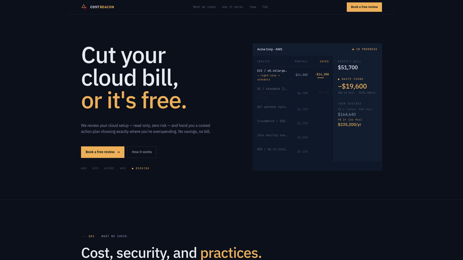
The engagement works the way this playbook is structured, prioritized by impact, not effort. A combination of AI-driven analysis with hands-on review of clusters, Spectrum usage, WLM configuration, and reserved capacity can produce a ranked action plan showing expected savings per item, alongside any security gaps discovered during the audit. Clients receive a prioritized action plan and may have the option to obtain implementation support if they prefer to hand off the tactical work.

The service may operate on a no upfront fee or retainer basis, invoicing a percentage of realized savings, maintaining alignment of incentives with outcomes rather than billable hours. If your Redshift bill has crept up without a clear explanation, start a pay-on-savings audit with Cost Beacon and get the prioritized list before your next invoice lands.

Sources

• Amazon Redshift Advisor documentation
• Optimize your workloads with Amazon Redshift Serverless AI-driven scaling and optimization | AWS Big Data Blog
• Redshift Spectrum query charges (AWS Knowledge Center)