30–60% DynamoDB Savings: Audit Ready for Engineering Teams

The fastest way to cut a DynamoDB bill is to combine four levers: review capacity mode, reserve baseline throughput where usage is steady, audit and prune GSIs, and move cold tables to Standard-IA. Together they typically bring 30% to 60% savings, but you need one diagnostic first: pull 30 days of consumed versus provisioned capacity per table in Cost Explorer or the AWS Pricing Calculator, and let that number tell you which lever to pull first.

---

TL;DR:

• Run 30 days of capacity usage data to identify whether to prioritize reservations, capacity mode, or table class changes for optimal savings.
• Reserve capacity based on the 30th percentile of past baseline usage, and compare reserved versus on-demand costs before committing.
• Migrate cold, infrequently accessed tables to Standard-IA only if storage costs significantly outweigh request costs over a 30-60 day window.
• Audit global secondary indexes and item sizes regularly to eliminate wasteful indexes and reduce write and read request units.
• Model regional table replication and transfer costs carefully, and keep compute resources local to optimize data transfer expenses.

---

Table of Contents

• How do you choose between on-demand and provisioned capacity?
• When should you move tables to Standard-IA?
• What data-model changes cut RCUs and WCUs fastest?
• What should you measure before you change anything?
• How do you control backup and PITR costs?
• How do transactional and burst workloads affect your bill?
• How do you write queries that consume fewer request units?
• How do you keep global tables cost-effective?
• What network data transfer costs should you watch?
• How do you minimize GSI costs without losing query flexibility?
• Cost Beacon’s take: when a runbook isn’t enough
• Get an outside read on your DynamoDB bill
• Sources

How do you choose between on-demand and provisioned capacity?

Billing mechanics decide this, not preference. On-demand charges you per read and write request with no capacity planning. Provisioned mode charges an hourly rate for capacity you reserve in advance, whether you use it or not. The break point comes down to utilization: if your table’s actual traffic runs well below what you’d need to provision for peak, on-demand usually wins. Above that, provisioned mode (especially with reservations) gets cheaper fast.

AWS’s own developer guide puts it plainly: on-demand suits unpredictable traffic, provisioned suits predictable steady throughput. The trap most teams fall into is leaving autoscaling targets too conservative, say 70% utilization headroom, out of fear of throttling. That fear is usually outdated. Modern autoscaling reacts within minutes, and pushing your target utilization from 70% up toward 80-90% often eliminates a large chunk of wasted provisioned capacity without triggering throttles, as long as your traffic doesn’t spike in seconds rather than minutes.

Reserved provisioned capacity changes the math further. You commit to a baseline amount of read or write capacity, purchased in 100-unit increments, for a one-year or three-year term, with options for partial or full upfront payment. Commitments are single-region and account-scoped.

Pro Tip: Size your reservation to the 30th percentile of your last 90 days of baseline usage, not the average. This avoids paying for capacity you won’t consistently use while still capturing most of the discount.

According to AWS pricing documentation, reserved capacity can significantly cut provisioned costs on one-year or three-year commitments. Database Savings Plans offer a more flexible alternative, spanning multiple database services and regions, though usually at a smaller discount than a dedicated reservation.

Run this checklist before committing:

1. Pull 90 days of ConsumedWriteCapacityUnits and ConsumedReadCapacityUnits against provisioned levels.
2. Identify your steady-state floor, ignoring short seasonal spikes.
3. Compare the reservation’s break-even point against on-demand pricing for that same floor.
4. Only reserve the portion of capacity you’d otherwise provision anyway. Never reserve peak.

When should you move tables to Standard-IA?

Table class selection hinges on one ratio: how much of your monthly bill comes from storage versus requests. DynamoDB Standard-IA cuts storage costs substantially compared to Standard, but it raises per-request costs moderately, according to AWS’s Database Blog. That trade only pays off when storage, not requests, dominates your spend.

Here’s the math on a typical time-series table: say a logging table holds 2 TB of data and generates modest read traffic, maybe 50 RCUs of steady demand. On Standard, storage might account for a large share of that table’s monthly cost.

The break-even rule of thumb involves comparing storage cost relative to provisioned throughput. When storage cost per unit of throughput is high, meaning you’re paying mostly to hold data rather than serve it, Standard-IA wins.

Good candidates and migration patterns:

• Historical or archival tables where reads are rare and mostly analytical.
• Log tables using monthly time-based partitioning, since old month-tables can flip to Standard-IA automatically once they age out of active writes.
• Tables you’ve already confirmed via Cost Explorer show storage cost consistently outweighing request cost over a 30 to 60-day window.

Validate every candidate in Cost Explorer before switching. A table that looks “cold” from the application layer sometimes carries hidden background read traffic from a batch job you forgot about.

What data-model changes cut RCUs and WCUs fastest?

Global secondary indexes are usually the biggest hidden cost driver on a DynamoDB bill. Every GSI write is billed as an additional write against the base table, so a table with three GSIs can multiply your effective write cost by four before you’ve touched a single line of application logic. Audit your indexes: pull ConsumedWriteCapacityUnits per GSI and cross-reference against actual query patterns in your application code. Indexes nobody queries, often left behind after a feature was deprecated, are pure waste. Removing them is one of the few genuinely code-free savings moves available.

Item size matters more than most teams realize. DynamoDB bills in fixed increments: 1 KB for writes, 4 KB for strongly consistent reads (with eventually consistent reads billed at half that rate). An item that’s 1.1 KB gets billed as if it were 2 KB. Shortening attribute names, from customer_purchase_timestamp to cts, for instance, plus compressing large text blobs and offloading anything over a few KB to S3 with a pointer stored in the item, keeps you under those billing boundaries.

Consistency choices carry real weight too. Eventually consistent reads cost half as much as strongly consistent reads. If your use case can tolerate a few hundred milliseconds of replication lag, which most dashboards, analytics views, and non-critical reads can, switching the default saves money on every single read. Reserve strongly consistent reads and transactional APIs for the operations that genuinely require them, like financial ledger updates or inventory locks.

Scans are the silent budget killer. A full table scan consumes capacity proportional to every item scanned, not just the ones returned. Replace recurring scans with:

• A Query operation against a proper partition key, whenever the access pattern allows it.
• Scheduled export-to-S3 jobs for analytics workloads, keeping DynamoDB itself for operational reads only.
• A secondary index designed specifically for the query pattern that currently forces a scan.

Pro Tip: If you’re scanning a table more than once a day for reporting, that’s a signal to build a dedicated GSI or move the workload to S3 and Athena instead.

TTL rounds out the list. Enabling time-to-live deletes expired items without consuming any write capacity, and you can stream those expiring items into S3 via Kinesis for archival before they’re purged. Expect deletion within 48 hours of expiry, not instantly, so don’t rely on TTL for hard real-time cleanup requirements.

What should you measure before you change anything?

Every optimization above depends on trustworthy data. Guessing at utilization is how teams end up over-provisioning “just in case” or under-reserving and paying full on-demand rates for predictable load.

Start with CloudWatch. The metrics that actually matter for cost decisions are ConsumedWriteCapacityUnits, ConsumedReadCapacityUnits, ProvisionedWriteCapacityUnits, ThrottledRequests, and SuccessfulRequestLatency, all documented in AWS’s usage pattern guide. Build a histogram of consumed versus provisioned capacity over 30 to 90 days per table; that single chart tells you whether you’re over-provisioned, under-provisioned, or roughly right.

1. Enable Cost and Usage Reports (CUR) and tag every table by team, environment, and application so costs can be attributed accurately.
2. Filter Cost Explorer by those tags to see storage-versus-throughput share per table, which drives your Standard-IA decisions.
3. Feed your proposed changes (a reservation, a table-class switch, a new autoscaling target) into the AWS Pricing Calculator to model dollar impact before you touch production.
4. Set a monthly reporting cadence and automated CloudWatch alarms for utilization drift, so a sudden traffic pattern change doesn’t quietly triple your bill before anyone notices.

Treat this measurement layer as non-negotiable groundwork. Every dollar figure in a reservation or migration decision should trace back to a specific CloudWatch metric or CUR line item, not a hunch.

How do you control backup and PITR costs?

Point-in-time recovery (PITR) and on-demand backups both add continuous storage cost on top of your table’s base storage, and that cost scales with table size, not usage. For production tables holding critical data, PITR is worth the expense. For everything else, it’s often dead weight.

• Disable PITR on development and staging tables; you rarely need to restore a test environment to an exact second.
• Use scheduled, less frequent backups for non-production tables instead of continuous PITR, and shorten retention windows.
• For large archival needs, export to S3 rather than relying on DynamoDB backups indefinitely. It’s cheaper long-term storage and keeps your table’s operational footprint lean.
• Review backup retention quarterly. Old backups nobody has restored in a year are a clear signal to prune.

How do transactional and burst workloads affect your bill?

Transactional APIs (TransactWriteItems, TransactGetItems) consume roughly double the capacity units of standard operations, because DynamoDB has to coordinate atomicity across items. Using transactions where a simple conditional write would do is a common and expensive habit. Reserve transactional APIs for cases that genuinely need all-or-nothing guarantees, like a payment ledger update paired with an inventory decrement.

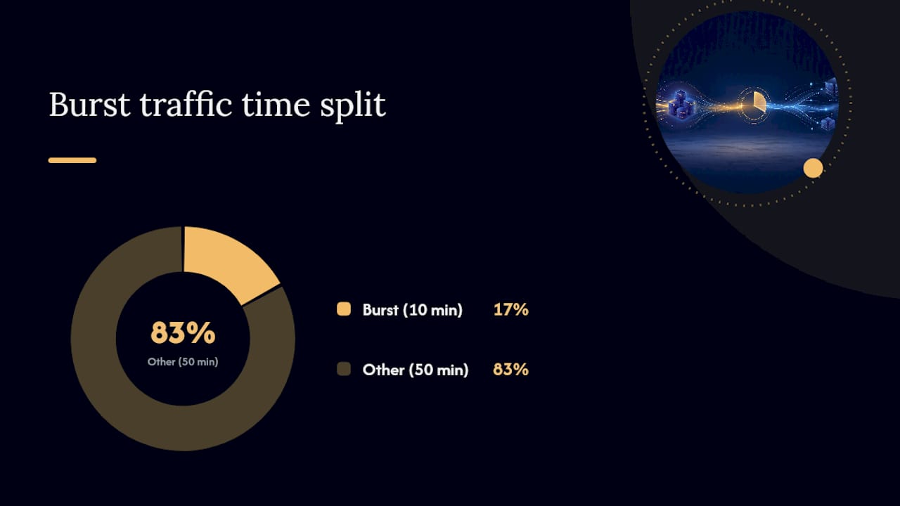
Burst traffic creates a different problem: it pushes you toward over-provisioning to survive the peak, even though average utilization stays low. If your traffic spikes for 10 minutes every hour, provisioning for that spike around the clock wastes capacity for the other 50 minutes.

Smoothing strategies that actually work:

• Introduce a queue (SQS) in front of write-heavy endpoints, so DynamoDB sees a steadier, buffered stream of writes instead of the raw burst.
• Batch writes where your application logic allows it. BatchWriteItem doesn’t reduce total capacity consumed, but it reduces round trips and helps smooth client-side request patterns.
• Lean on autoscaling with a higher target utilization for workloads with gradual (minutes, not seconds) traffic growth, but keep on-demand mode for workloads with genuinely unpredictable, spiky patterns that autoscaling can’t react to fast enough.
• Separate your hot, latency-sensitive tables from your bulk, less time-sensitive ones, so a burst on one doesn’t force you to over-provision the other.

How do you write queries that consume fewer request units?

Query efficiency comes down to designing for your actual access patterns instead of your data model’s convenience. A well-designed partition key that matches your most frequent query eliminates scans entirely, which is the single biggest request-unit saver available.

A few habits separate efficient DynamoDB usage from expensive DynamoDB usage:

• Project only the attributes you need in a GSI, rather than projecting the entire item; smaller projections mean lower index write costs and smaller query payloads.
• Use Query with a sort-key condition instead of pulling a full partition and filtering client-side. A filter expression still consumes capacity for every item read, not just the ones returned.
• Batch reads and writes with BatchGetItem and BatchWriteItem wherever your application logic supports it, reducing overhead from repeated round trips.
• Cache frequently read, rarely changed items (configuration values, reference data) in something like DAX or an application-layer cache, so DynamoDB isn’t serving the same read over and over.
• Default to eventually consistent reads unless a specific operation requires strong consistency, since it halves read capacity consumption on every call.

None of these require a schema redesign. They’re query-pattern discipline, and they’re usually the fastest wins available to a team that hasn’t touched its access patterns since the original build.

How do you keep global tables cost-effective?

Global tables replicate every write to every region you add, which means adding a region doesn’t just add latency benefits, it multiplies your write costs by the number of replica regions. A table replicated across three regions pays for three times the write capacity of a single-region table.

The fix isn’t avoiding global tables, it’s being deliberate about which tables actually need global replication. Session data, regional caches, and anything that doesn’t need to survive a full regional outage usually doesn’t belong in a multi-region setup. Reserve global tables for data where cross-region availability or low-latency local reads genuinely matter to the business, like a user profile that needs to load fast for customers on three continents.

Region count matters more than most teams initially budget for. Before adding a third or fourth replica region, model the write-cost multiplier against actual latency or availability requirements. Two regions often satisfies disaster-recovery needs at half the replication cost of four. Also audit whether every region actually receives meaningful read traffic. A replica region added years ago for a market you no longer serve is a quiet, ongoing cost with zero benefit.

What network data transfer costs should you watch?

DynamoDB itself doesn’t charge for data transfer within the same region between DynamoDB and most AWS services, but cross-region and internet-bound transfer both carry charges that add up quietly on high-traffic tables. Global tables are the most common source: every replicated write crosses a region boundary, and that transfer is billed separately from the write-capacity cost itself.

Cross-AZ traffic within a region is typically not a major line item for DynamoDB specifically, but if your application architecture routes reads through a Lambda function or EC2 instance in a different AZ before returning data to the client, you’re paying transfer costs that have nothing to do with DynamoDB’s own pricing. Keep compute close to the table’s region, and check whether VPC endpoints for DynamoDB are configured to avoid unnecessary transfer through a NAT gateway, which can add unexpected cost for high-volume workloads.

How do you minimize GSI costs without losing query flexibility?

Every GSI write bills against the base table, so the honest first step is asking whether you need the index at all. Pull consumed capacity per GSI over 30 days and compare it against actual query logs. An index with high write cost and near-zero query volume is pure liability.

Where a GSI is genuinely needed, keep its projection lean. Projecting ALL attributes into every index multiplies storage and can inflate query costs when you only ever need three fields back. Sparse indexes, where only a subset of items contain the indexed attribute, are worth using deliberately: they keep the index smaller and cheaper without sacrificing the query pattern you actually need.

Consolidate where you can. Two narrow, overlapping GSIs built at different points in a project’s history can often merge into one composite index with a smarter sort key, cutting both write and storage cost in half for that access pattern.

Cost Beacon’s take: when a runbook isn’t enough

Most of the levers above are things any competent engineering team can execute internally over a couple of sprints. Cost Beacon’s audit process combines AI-driven analytics with hands-on engineering review specifically because the hardest part usually isn’t knowing the levers, it’s finding which tables and accounts actually need them across dozens or hundreds of tables spread over multiple AWS accounts.

We work on a pay-on-savings basis: no upfront fee, no retainer, you pay a percentage of what’s actually realized.

An internal runbook works well for a single team with a handful of tables. A paid review earns its cost when you’re running a multi-account AWS organization, seeing unpredictable spend spikes nobody can explain, or simply don’t have the engineering bandwidth to audit every GSI and table class decision this quarter.

— Aaditya Parashar

Get an outside read on your DynamoDB bill

The levers in this guide handle the fixes your team can execute directly. What’s harder to do internally is finding every idle table, orphaned GSI, and misconfigured backup policy across a sprawling multi-account setup while still shipping product features. Cost Beacon is built for exactly that gap: an AI-driven analytics pass combined with hands-on engineering review across your AWS, GCP, Azure, or Kubernetes environments, delivered as a prioritized action plan with expected savings per item.

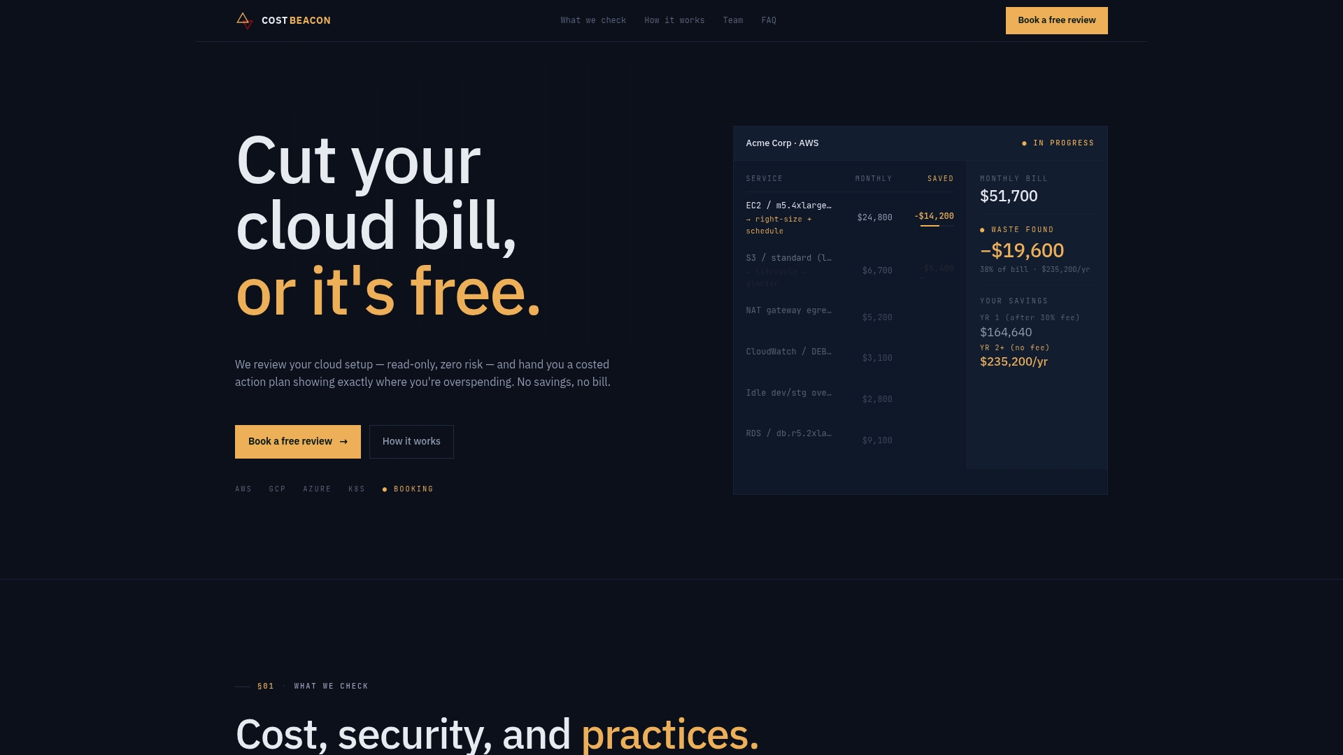
There’s no upfront fee. Cost Beacon works on a pay-on-savings basis, so the incentive is aligned with your outcome from day one, not ours. If you’re managing DynamoDB spend across a multi-account AWS organization and suspect there’s more waste than your team has time to chase down, start a cloud cost and security review with Cost Beacon and see what a prioritized savings plan looks like for your actual infrastructure.

Recommended

• Pay-on-savings cloud cost & security review